In this example, we describe the coupling between two standard gain horn antennas. Several cases are considered.
Zero movement definitions (Figure 1a). The antennas are looking face-to-face.
One movement definition (Figure 1b). The receiving antenna is rotated around antenna boresight. The coupling is evaulated at for rotation angles between 0° (brown; just like in Figure 1a), 30° (not shown), 60° (not shown), and 90° (white).
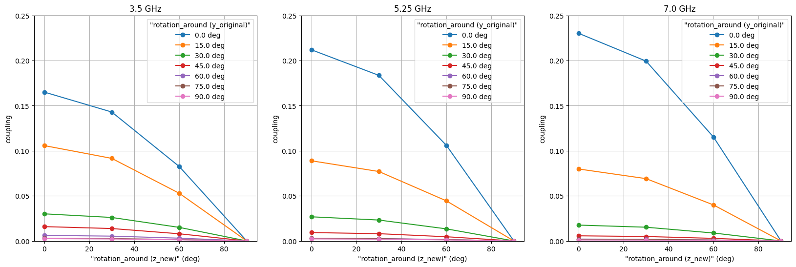
Two movement definitions (Figure 1c). Firsly, the receiving antenna is rotated around the transmitting antenna (gray arrow), described by the zenith angle . The coupling is evaluated at the angles . For each of these position, the receiving antenna is also moved around its boresight, just like in Figure 1b. For the initial position, this is illustrated by the white antenna. For the remaining positions, the rotated antenna is not drawn.
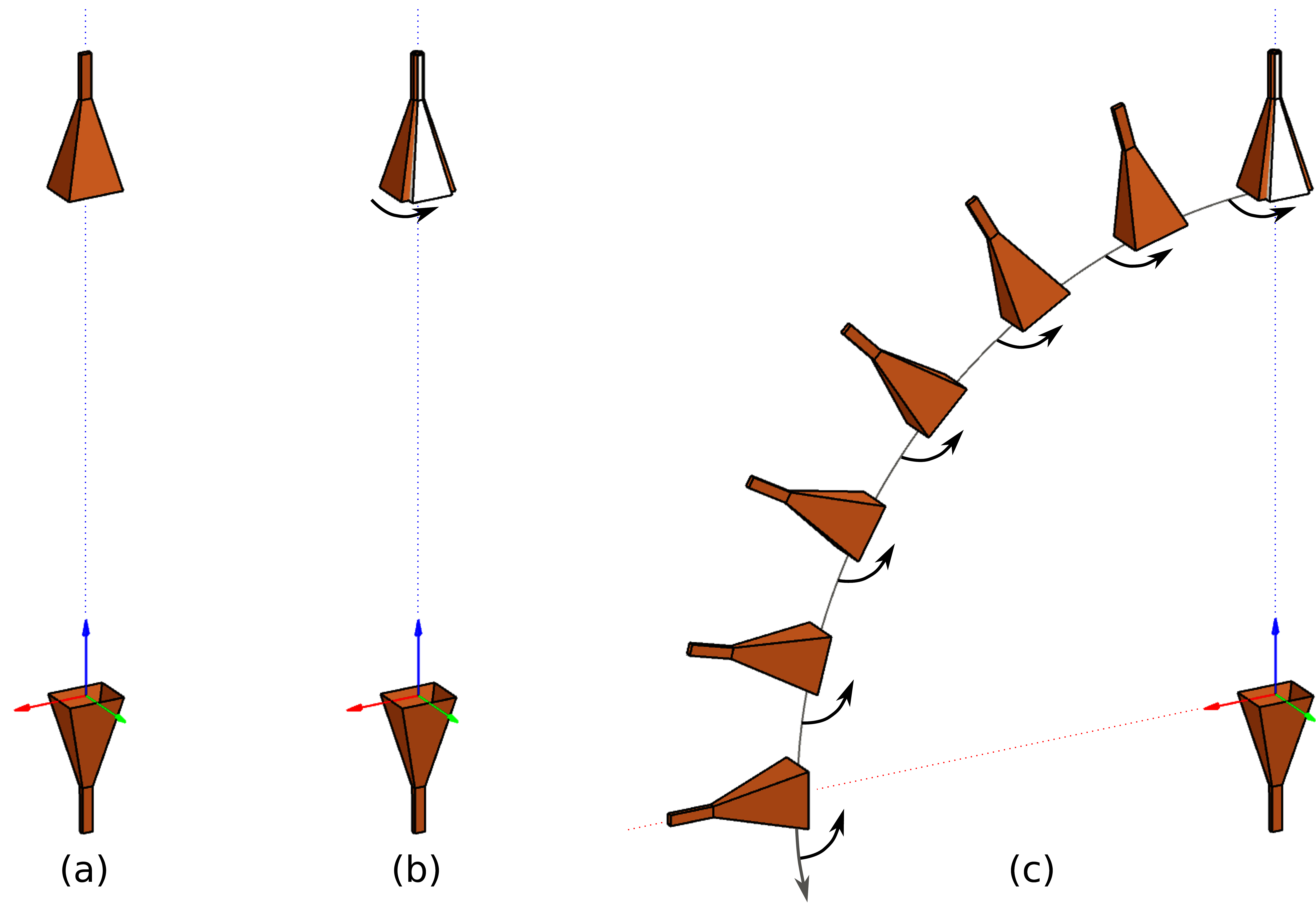
Figure 1:Example setup for antenna coupling simulation with GRASP from TICRA. Three setups are illustrated, corresponding to zero (a), one (b), and two movement definitions (c).
Imports and definitions for easy plotting
# import python libraries/modules
import os
import pint # for unit conversion when plotting
import numpy as np
import matplotlib.pyplot as plt

# import functions from pycra-tools
from pycra_tools import readcut_coupling, torfile

# function docstrings are available as follows:
# print(readcut_coupling.__doc__)
# print(torfile.__doc__)
Read data from files
directory_example_simulation = '/home/phjschmid/phdphysics/simulation/projects/pycra_tools/coupling_example'
torfilepath = os.path.join(directory_example_simulation, 'Job_01', 'Job_01.tor')
cutfilepath0 = os.path.join(directory_example_simulation, 'Job_01', 'coupling_system_rx_zero.cut')
cutfilepath1 = os.path.join(directory_example_simulation, 'Job_01', 'coupling_system_rx_one.cut')
cutfilepath2 = os.path.join(directory_example_simulation, 'Job_01', 'coupling_system_rx_two.cut')

# read files
tordict = torfile.tor2dict(torfilepath)
da0 = readcut_coupling(cutfilepath=cutfilepath0, tordict=tordict)
da1 = readcut_coupling(cutfilepath=cutfilepath1, tordict=tordict)
da2 = readcut_coupling(cutfilepath=cutfilepath2, tordict=tordict)
Inspect structure of the dataframes
print('# print(da0)')
print(da0)
print('\n\n# print(da0.name)')
print(da0.name)
print('\n\n# print(da0.freq)')
print(da0.freq)
# print(da0)
<xarray.DataArray '/home/phjschmid/phdphysics/simulation/projects/pycra_tools/coupling_example/Job_01/coupling_system_rx_zero.cut' (
freq: 3)> Size: 48B
array([-0.00248305-0.16498349j, 0.21188705+0.00160079j,
-0.01177798+0.22985868j])
Coordinates:
* freq (freq) float64 24B 3.5e+09 5.25e+09 7e+09
Attributes:
file_format: cuts
class_name: coupling_system
receiver_sources: ['rectangular_horn_rx']
amplitude_only: off
movement_definition: None
cqlist: off
comment: None
# print(da0.name)
/home/phjschmid/phdphysics/simulation/projects/pycra_tools/coupling_example/Job_01/coupling_system_rx_zero.cut
# print(da0.freq)
<xarray.DataArray 'freq' (freq: 3)> Size: 24B
array([3.50e+09, 5.25e+09, 7.00e+09])
Coordinates:
* freq (freq) float64 24B 3.5e+09 5.25e+09 7e+09
Attributes:
long_name: frequency
units: Hz
print('# print(da1)')
print(da1)
print('\n\n# print(da1.name)')
print(da1.name)
print('\n\n# print(da1.freq)')
print(da1.freq)
print('\n\n# print(da1.m1)')
print(da1.m1)
# print(da1)
<xarray.DataArray '/home/phjschmid/phdphysics/simulation/projects/pycra_tools/coupling_example/Job_01/coupling_system_rx_one.cut' (
freq: 3,
m1: 4)> Size: 192B
array([[-2.48304943e-03-1.64983493e-01j, -2.15038389e-03-1.42879896e-01j,
-1.24152472e-03-8.24917463e-02j, 4.75757215e-17+7.21852018e-18j],
[ 2.11887051e-01+1.60078640e-03j, 1.83499569e-01+1.38632169e-03j,
1.05943525e-01+8.00393198e-04j, 4.69455635e-17+8.56322568e-17j],
[-1.17779783e-02+2.29858679e-01j, -1.02000285e-02+1.99063455e-01j,
-5.88898917e-03+1.14929340e-01j, -2.39144714e-18+3.16118334e-16j]])
Coordinates:
* freq (freq) float64 24B 3.5e+09 5.25e+09 7e+09
* m1 (m1) float64 32B 0.0 30.0 60.0 90.0
Attributes:
file_format: cuts
class_name: coupling_system
receiver_sources: ['rectangular_horn_rx']
amplitude_only: off
movement_definition: movement_definition_rx_one
cqlist: off
comment: None
# print(da1.name)
/home/phjschmid/phdphysics/simulation/projects/pycra_tools/coupling_example/Job_01/coupling_system_rx_one.cut
# print(da1.freq)
<xarray.DataArray 'freq' (freq: 3)> Size: 24B
array([3.50e+09, 5.25e+09, 7.00e+09])
Coordinates:
* freq (freq) float64 24B 3.5e+09 5.25e+09 7e+09
Attributes:
long_name: frequency
units: Hz
# print(da1.m1)
<xarray.DataArray 'm1' (m1: 4)> Size: 32B
array([ 0., 30., 60., 90.])
Coordinates:
* m1 (m1) float64 32B 0.0 30.0 60.0 90.0
Attributes:
long_name: rotation_around (z_original)
name: rotation_around (z_original)
units: deg
print('# print(da2)')
print(da2)
print('\n\n# print(da2.name)')
print(da2.name)
print('\n\n# print(da2.freq)')
print(da2.freq)
print('\n\n# print(da2.m1)')
print(da2.m1)
print('\n\n# print(da2.m2)')
print(da2.m2)
# print(da2)
<xarray.DataArray '/home/phjschmid/phdphysics/simulation/projects/pycra_tools/coupling_example/Job_01/coupling_system_rx_two.cut' (
freq: 3,
m1: 7,
m2: 4)> Size: 1kB
array([[[-2.48304943e-03-1.64983493e-01j,
-2.15038389e-03-1.42879896e-01j,
-1.24152472e-03-8.24917463e-02j,
4.75757215e-17+7.21852018e-18j],
[ 1.48517648e-02-1.04625827e-01j,
1.28620056e-02-9.06086240e-02j,
7.42588238e-03-5.23129134e-02j,
2.59070547e-17+3.01849777e-17j],
[ 2.53641241e-02-1.60862233e-02j,
2.19659758e-02-1.39310780e-02j,
1.26820621e-02-8.04311164e-03j,
1.16416316e-18+1.20087308e-17j],
[ 1.08795627e-02+1.15407139e-02j,
9.42197769e-03+9.99455146e-03j,
5.43978136e-03+5.77035697e-03j,
1.73904875e-18-6.15850079e-18j],
[-5.16611446e-04+6.11390793e-03j,
-4.47398636e-04+5.29479958e-03j,
-2.58305723e-04+3.05695396e-03j,
-8.67982156e-18-1.21707225e-17j],
...
[ 1.39397997e-02-1.06585942e-02j,
1.20722206e-02-9.23061338e-03j,
6.96989984e-03-5.32929712e-03j,
-3.25434783e-17-7.23221678e-17j],
[-4.72514398e-03+3.13070223e-03j,
-4.09209472e-03+2.71126767e-03j,
-2.36257199e-03+1.56535112e-03j,
-2.09229321e-18-1.31877321e-17j],
[ 9.45057740e-04-1.80216342e-03j,
8.18444011e-04-1.56071931e-03j,
4.72528870e-04-9.01081711e-04j,
-1.13878789e-17+1.35449776e-17j],
[ 1.84267059e-03+5.20571432e-04j,
1.59579954e-03+4.50828085e-04j,
9.21335295e-04+2.60285716e-04j,
-8.81949650e-18+2.18389998e-17j],
[ 8.05691312e-04+6.67543953e-04j,
6.97749143e-04+5.78110022e-04j,
4.02845656e-04+3.33771977e-04j,
-1.58117891e-18-1.46989433e-17j]]])
Coordinates:
* freq (freq) float64 24B 3.5e+09 5.25e+09 7e+09
* m1 (m1) float64 56B 0.0 15.0 30.0 45.0 60.0 75.0 90.0
* m2 (m2) float64 32B 0.0 30.0 60.0 90.0
Attributes:
file_format: cuts
class_name: coupling_system
receiver_sources: ['rectangular_horn_rx']
amplitude_only: off
movement_definition: movement_definition_rx_two
cqlist: off
comment: None
# print(da2.name)
/home/phjschmid/phdphysics/simulation/projects/pycra_tools/coupling_example/Job_01/coupling_system_rx_two.cut
# print(da2.freq)
<xarray.DataArray 'freq' (freq: 3)> Size: 24B
array([3.50e+09, 5.25e+09, 7.00e+09])
Coordinates:
* freq (freq) float64 24B 3.5e+09 5.25e+09 7e+09
Attributes:
long_name: frequency
units: Hz
# print(da2.m1)
<xarray.DataArray 'm1' (m1: 7)> Size: 56B
array([ 0., 15., 30., 45., 60., 75., 90.])
Coordinates:
* m1 (m1) float64 56B 0.0 15.0 30.0 45.0 60.0 75.0 90.0
Attributes:
long_name: rotation_around (y_original)
name: rotation_around (y_original)
units: deg
# print(da2.m2)
<xarray.DataArray 'm2' (m2: 4)> Size: 32B
array([ 0., 30., 60., 90.])
Coordinates:
* m2 (m2) float64 32B 0.0 30.0 60.0 90.0
Attributes:
long_name: rotation_around (z_new)
name: rotation_around (z_new)
units: deg
Visualize data
Let us plot the data that is stored in the three dataframes discussed above. For simplifying the comparison, let us choose the same axis for all the figures.
# chose common axis limits for all plots
ymax = (1+max(np.abs(da0).max(),np.abs(da1).max(),np.abs(da2).max())//0.05)*0.05
ylims = [0,ymax]

# prepare unit conversion tool
ureg = pint.UnitRegistry()
Zero movement defintions
# zero movement definitions (face-to-face coupling)
fig, ax = plt.subplots()
ax.plot([(freq * ureg[da1.freq.units]).to('GHz').magnitude for freq in da0.freq.values], np.abs(da0.data), marker='o')
ax.grid(True, which='major', axis='both')
ax.set_ylim(ylims)
ax.set_xlabel(f'{da0.freq.long_name} (GHz)')
ax.set_ylabel('coupling')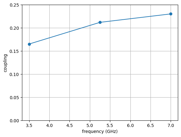
One movement defintion
fig, ax = plt.subplots()
ax.set_xlabel(f'"{da1.m1.long_name}" ({da1.m1.units})')
ax.set_ylabel('coupling')
ax.grid(True, which='major', axis='both')
for freq in da1.freq.values:
    freqGHz = (freq * ureg[da1.freq.units]).to('GHz').magnitude
    ax.plot(da1.sel(freq=freq).m1.values, np.abs(da1.sel(freq=freq).data), marker='o',
            label=f'{freqGHz} GHz')
ax.set_ylim(ylims)
ax.legend(title=da1.freq.long_name)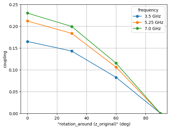
Two movement defintions
freq = da2.freq.values[0]
fig, ax = plt.subplots(1,3,figsize=(6*3+2,6))
for ii,freq in enumerate(da2.freq.values):
    ax[ii].set_title(f"{(freq * ureg[da2.freq.units]).to('GHz').magnitude} GHz")
    ax[ii].set_xlabel(f'"{da2.m2.long_name}" ({da2.m2.units})')
    ax[ii].set_ylabel('coupling')
    ax[ii].grid(True, which='major', axis='both')
    for m1 in da2.m1.values:
        ax[ii].plot(da2.sel(freq=freq, m1=m1).m2.values, np.abs(da2.sel(freq=freq, m1=m1).data), marker='o',
                    label=f'{m1} {da2.m1.units}')
    ax[ii].set_ylim(ylims)
    ax[ii].legend(title=f'"{da2.m1.long_name}"')
plt.show()