Let us show how pycra-tools is used for reading field data from GRASP. To this end, let us consider the basic example illustrated Figure 1. The figure shows a rectangular horn antenna (brown), in the center of which there is a coordinate system with x-axis (red), y-axis (green) and z-axis (blue). Such antennas are used for many kinds of applications, see e.g. Schmid et al. (2025) for a usage related to weather radars. In the example presented here, we read data from near- and farfield Physical Optics simulations of the antenna radiation pattern.
In Figure 1, on the one hand, the turquoise color represents a nearfield spherical-class grid uv-type coordinate system, see e.g. TICRA (2024) manual p. 574, 2122, with coordinates
with zenith angle , azimuth angle , and given radius .
The three gray lines, on the other hand, represent farfield spherical-class cut with polar-type coordinate system (gray). The cuts are defined here in the “farfield” (infinitely far away from the antenna in GRASP's definition), but drawn at radius 1.5 m for illustration.
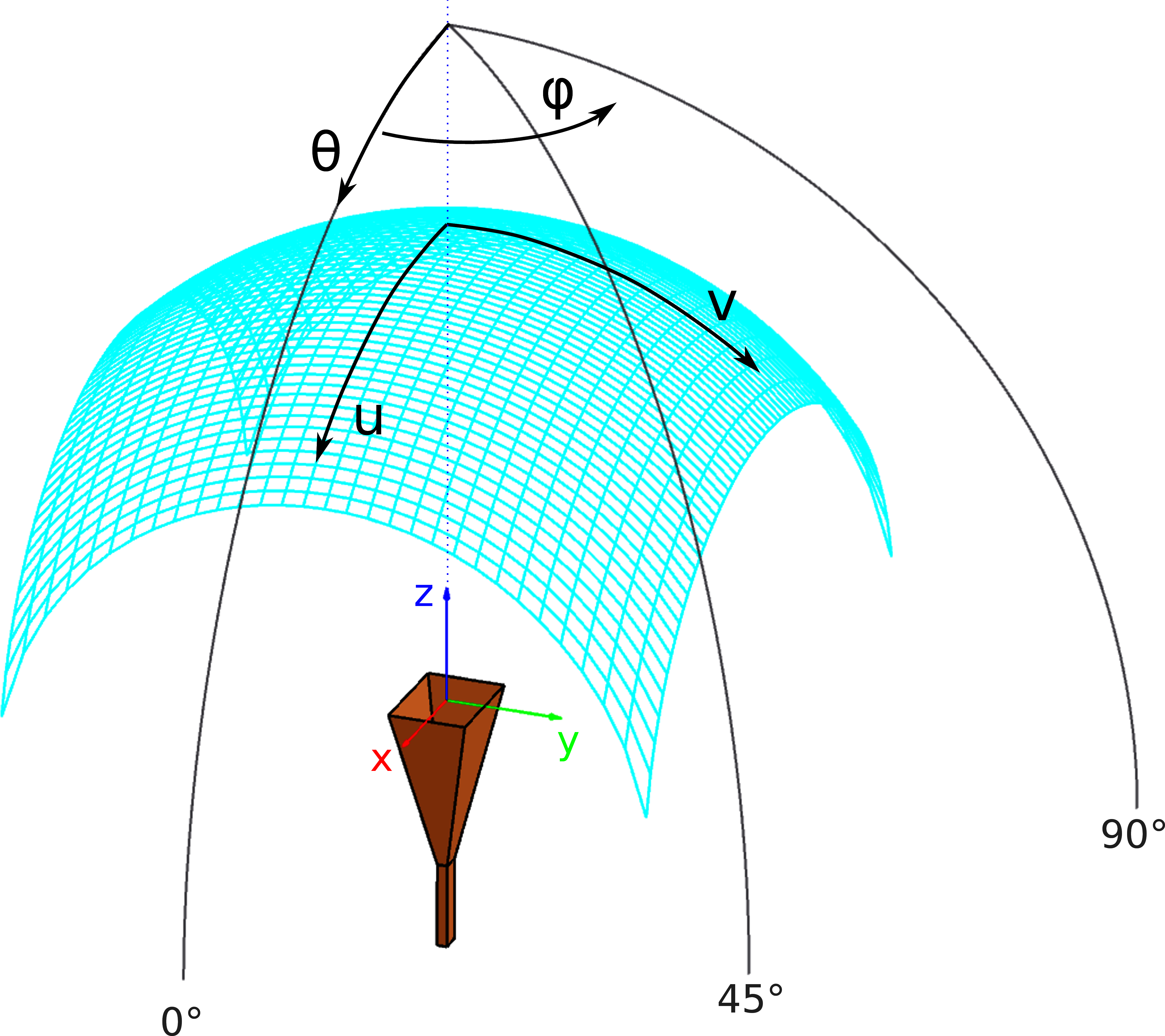
Figure 1:Example setup for antenna pattern simulation with GRASP from TICRA.
On the nearfield grid we evaluated the e_field (electric field), and on an identical grid also the h_field (magnetic field); both are needed to compute the intensity for instance.
On the farfield cuts we only simulated the electric field, from which one can calculate the antenna directivity, for example. The linear “polarization” definition was chosen in all cases.
Imports and definitions for easy plotting
# import python libraries/modules
import os
import numpy as np
import matplotlib as mpl
import matplotlib.pyplot as plt
from mpl_toolkits.axes_grid1 import make_axes_locatable

# import functions from pycra-tools
from pycra_tools import readcut, readgrid, torfile

# function docstrings are available as follows:
# print(readcut.__doc__)
# print(readgrid.__doc__)
# print(torfile.__doc__)

# auxiliary function for plotting data in cuts
def cutplot_magnitudes(da):
    """
    Auxiliary function for plotting 1D field data for one frequency.

    Args:
        da (<class 'xarray.core.dataarray.DataArray'>):
            Xarray dataframe with one frequency only

    Returns:
        fig: figure handle
        ax: axis handle
    """

    nr_components = len(da.comp.values)
    fig, ax = plt.subplots(1, nr_components, figsize=(4*nr_components+2, 5))
    for ii,_ in enumerate(da.comp.values):
        ax[ii].set_xlabel(f"${da.Y.attrs['texname']}$ ({da.Y.attrs['units']})" if da.Y.attrs['units'] else da.Y.attrs['texname'])
        ax[ii].set_ylabel(f"${da.comp.attrs['names_math'][ii]}$ ({da.comp.attrs['units_math'][ii]})")
        for jj,xval in enumerate(da.X.values):
            ax[ii].plot(da.Y.values, np.abs(da.values)[:,jj,ii], label=f"{xval} {da.X.units}")
        ax[ii].legend()
        ax[ii].grid(True, which='major', axis='both')

    return fig, ax

# auxiliary function for plotting data in grids
def gridplot_magnitudes(da):
    """
    Auxiliary function for plotting 2D field data for one frequency.

    Args:
        da (<class 'xarray.core.dataarray.DataArray'>):
            Xarray dataframe with one frequency only

    Returns:
        fig: figure handle
        ax: axis handle
    """

    nr_components = len(da.comp.values)
    fig, ax = plt.subplots(1, nr_components, figsize=(4*nr_components+2, 5))
    for ii,_ in enumerate(da.comp.values):
        ax[ii].set_xlabel(f"{da.X.attrs['texname']} ({da.X.attrs['units']})" if da.X.attrs['units'] else da.X.attrs['texname'])
        ax[ii].set_ylabel(f"{da.Y.attrs['texname']} ({da.Y.attrs['units']})" if da.Y.attrs['units'] else da.Y.attrs['texname'])
        img = ax[ii].imshow(np.abs(da.values)[:,:,ii],
                        extent=[np.min(da.X.values), np.max(da.X.values),
                                np.min(da.Y.values), np.max(da.Y.values)],
                        vmin=None, vmax=None, cmap=mpl.colormaps['viridis'])
        divider = make_axes_locatable(ax[ii])
        cax = divider.append_axes("right", size="5%", pad=0.05)
        plt.colorbar(img, cax=cax)
        cax.set_ylabel(f"${da.comp.attrs['names_math'][ii]}$ ({da.comp.attrs['units_math'][ii]})")

    return fig, ax
Read data from files
To fully interpreting the numerical data stored in the .cut/.grd/.h5 files, some extra information may be needed, and which is normally stored in the .tor file (such as class information for nearfield .cut and .grd files, and frequency information for .cut files). Sometimes the required information is not stored in the .tor file either; for example, when the user did not explicitely associate frequency information with the objects during the simulation, then frequency must be retrieved from the .tci file (this is not yet implemented in pycra-tools though).
In such cases, or when the .tor file is not available, the information can also be provided manually by the user, using the input dictionary {userdict}.
The pycra-tools package combines the information, returning an Xarray labeled multi-dimensional array, denoted da_* in the code below.
# define filepaths
directory_example_simulation = '/home/phjschmid/phdphysics/simulation/projects/pycra_tools/fields_example'
torfilepath = os.path.join(directory_example_simulation, 'Job_01', 'Job_01.tor')
cutfilepath = os.path.join(directory_example_simulation, 'Job_01', 'spherical_cut_far_E.cut')
grdfilepath_efield = os.path.join(directory_example_simulation, 'Job_01', 'spherical_grid_uv_near_E.grd')
grdfilepath_hfield = os.path.join(directory_example_simulation, 'Job_01', 'spherical_grid_uv_near_H.grd')

# ------------------------------------------------------------------------------
# Method 1:
# - read information from torfile into dictionary
# - use this dictionary to read the cut/grid files
# ------------------------------------------------------------------------------

tordict = torfile.tor2dict(torfilepath)
da_cut_efield = readcut(cutfilepath=cutfilepath, tordict=tordict)
da_grid_efield = readgrid(gridfilepath=grdfilepath_efield, tordict=tordict)
da_grid_hfield = readgrid(gridfilepath=grdfilepath_hfield, tordict=tordict)

# ------------------------------------------------------------------------------
# Method 2:
# - pass torfilepath for reading the cut/grid files
# Remark: reading the torfile several times, this method is slower for multiple files.
# ------------------------------------------------------------------------------

# tordict = torfile.tor2dict(torfilepath)
# da_cut_efield = readcut(cutfilepath=cutfilepath, torfilepath=torfilepath)
# da_grid_efield = readgrid(gridfilepath=grdfilepath_efield, torfilepath=torfilepath)
# da_grid_hfield = readgrid(gridfilepath=grdfilepath_hfield, torfilepath=torfilepath)

# ------------------------------------------------------------------------------
# Method 3:
# - create dictionary with necessary information (class_name, field_type)
# - use this dictionary to read the cut/grid files
# Remark for .grd-files:
#   Sometimes the frequency information is given.
#   In this case, the user-frequencies are compared with the ones in the file.
# ------------------------------------------------------------------------------

# userdict = {
#     # 'class_name': 'spherical',
#     # 'field_type': 'e_field',
#     'coordinate_system_name': 'rectangular_horn_tx_coor_sys',
#     'field_region_distance_m': np.inf,
#     'freqs_Hz': np.linspace(3.5,7,5)*1e9}
# da_cut_efield = readcut(cutfilepath=cutfilepath, userdict=userdict)

# userdict = {
#     'class_name': 'spherical',
#     # 'field_type': 'e_field',
#     'coordinate_system_name': 'rectangular_horn_tx_coor_sys',
#     'field_region_distance_m': 1,
#     'freqs_Hz': np.linspace(3.5,7,5)*1e9}
# da_grid_efield = readgrid(gridfilepath=grdfilepath_efield, userdict=userdict)

# userdict = {
#     'class_name': 'spherical',
#     'field_type': 'h_field',
#     'coordinate_system_name': 'rectangular_horn_tx_coor_sys',
#     'field_region_distance_m': 1,
#     'freqs_Hz': np.linspace(3.5,7,5)*1e9}
# da_grid_hfield = readgrid(gridfilepath=grdfilepath_hfield, userdict=userdict)
Inspect structure of the dataframes
print('# print(da_cut_efield)')
print(da_cut_efield)
print('\n\n# print(da_cut_efield.name)')
print(da_cut_efield.name)
print('\n\n# print(da_cut_efield.X)')
print(da_cut_efield.X)
print('\n\n# print(da_cut_efield.Y)')
print(da_cut_efield.Y)
print('\n\n# print(da_cut_efield.comp)')
print(da_cut_efield.comp)
print('\n\n# print(da_cut_efield.freq)')
print(da_cut_efield.freq)
# print(da_cut_efield)
<xarray.DataArray '/home/phjschmid/phdphysics/simulation/projects/pycra_tools/fields_example/Job_01/spherical_cut_far_E.cut' (
Y: 101,
X: 3,
comp: 2,
freq: 5)> Size: 48kB
array([[[[ 1.74484242e-15+1.45514118e-15j,
-5.75629720e-15-1.71494957e-14j,
-1.34395723e-16-7.33644272e-16j,
-9.37114725e-16-5.93612733e-15j,
-1.99469269e-15-5.57723944e-15j],
[ 2.69564812e+00+6.56589587e+00j,
4.02833236e+00+7.64269604e+00j,
5.51903066e+00+8.43651105e+00j,
7.08609949e+00+8.90764531e+00j,
8.65399921e+00+9.05332324e+00j]],
[[ 1.74484242e-15+1.45514118e-15j,
-5.75629720e-15-1.71494957e-14j,
-1.34395723e-16-7.33644272e-16j,
-9.37114725e-16-5.93612733e-15j,
-1.99469269e-15-5.57723944e-15j],
[ 2.69564812e+00+6.56589587e+00j,
4.02833236e+00+7.64269604e+00j,
5.51903066e+00+8.43651105e+00j,
7.08609949e+00+8.90764531e+00j,
...
9.75601549e-05+1.56524489e-04j,
-1.68909665e-05-4.77115418e-05j,
5.94350049e-05-2.87865915e-05j,
5.52580894e-06+3.31317751e-05j],
[ 8.49114215e-02+1.76901478e-03j,
1.68573931e-02+2.70462831e-02j,
-4.20691472e-03-1.19243579e-02j,
2.02435577e-02-9.80441192e-03j,
2.50352435e-03+1.45603783e-02j]],
[[-3.30670906e-16+8.60016882e-17j,
6.03660501e-16-1.88525779e-16j,
5.57744339e-16-7.20107852e-18j,
-2.64168881e-16+1.90958421e-16j,
-2.73812326e-16+6.36782472e-16j],
[ 6.94736846e-03-1.66416447e-01j,
4.99815494e-01+3.16100200e-01j,
1.13624031e-01+1.72498103e-01j,
-5.46744716e-01-7.91788301e-02j,
-2.19435307e-01-1.08329944e-01j]]]], shape=(101, 3, 2, 5))
Coordinates:
* Y (Y) float64 808B 0.0 0.9 1.8 2.7 3.6 ... 86.4 87.3 88.2 89.1 90.0
* X (X) float64 24B 0.0 45.0 90.0
* comp (comp) <U1 8B 'a' 'b'
* freq (freq) float64 40B 3.5e+09 4.375e+09 5.25e+09 6.125e+09 7e+09
Attributes:
class_name: spherical
coordinate_system: polar
coordinate_system_name: rectangular_horn_tx_coor_sys
field_region_distance_m: inf
# print(da_cut_efield.name)
/home/phjschmid/phdphysics/simulation/projects/pycra_tools/fields_example/Job_01/spherical_cut_far_E.cut
# print(da_cut_efield.X)
<xarray.DataArray 'X' (X: 3)> Size: 24B
array([ 0., 45., 90.])
Coordinates:
* X (X) float64 24B 0.0 45.0 90.0
Attributes:
long_name: polar angle
texname: \phi
units: deg
# print(da_cut_efield.Y)
<xarray.DataArray 'Y' (Y: 101)> Size: 808B
array([ 0. , 0.9, 1.8, 2.7, 3.6, 4.5, 5.4, 6.3, 7.2, 8.1, 9. , 9.9,
10.8, 11.7, 12.6, 13.5, 14.4, 15.3, 16.2, 17.1, 18. , 18.9, 19.8, 20.7,
21.6, 22.5, 23.4, 24.3, 25.2, 26.1, 27. , 27.9, 28.8, 29.7, 30.6, 31.5,
32.4, 33.3, 34.2, 35.1, 36. , 36.9, 37.8, 38.7, 39.6, 40.5, 41.4, 42.3,
43.2, 44.1, 45. , 45.9, 46.8, 47.7, 48.6, 49.5, 50.4, 51.3, 52.2, 53.1,
54. , 54.9, 55.8, 56.7, 57.6, 58.5, 59.4, 60.3, 61.2, 62.1, 63. , 63.9,
64.8, 65.7, 66.6, 67.5, 68.4, 69.3, 70.2, 71.1, 72. , 72.9, 73.8, 74.7,
75.6, 76.5, 77.4, 78.3, 79.2, 80.1, 81. , 81.9, 82.8, 83.7, 84.6, 85.5,
86.4, 87.3, 88.2, 89.1, 90. ])
Coordinates:
* Y (Y) float64 808B 0.0 0.9 1.8 2.7 3.6 ... 86.4 87.3 88.2 89.1 90.0
Attributes:
long_name: zenith angle
texname: \theta
units: deg
# print(da_cut_efield.comp)
<xarray.DataArray 'comp' (comp: 2)> Size: 8B
array(['a', 'b'], dtype='<U1')
Coordinates:
* comp (comp) <U1 8B 'a' 'b'
Attributes:
long_name: field comopnents
field_type: e_field
polarisation: linear
names_math: ['E_{co}', 'E_{cx}']
units_math: ['W$^{0.5}$', 'W$^{0.5}$']
unitsystem: TICRA
# print(da_cut_efield.freq)
<xarray.DataArray 'freq' (freq: 5)> Size: 40B
array([3.500e+09, 4.375e+09, 5.250e+09, 6.125e+09, 7.000e+09])
Coordinates:
* freq (freq) float64 40B 3.5e+09 4.375e+09 5.25e+09 6.125e+09 7e+09
Attributes:
long_name: frequency
units: Hz
print('# print(da_grid_efield)')
print(da_grid_efield)
print('\n\n# print(da_grid_efield.name)')
print(da_grid_efield.name)
print('\n\n# print(da_grid_efield.X)')
print(da_grid_efield.X)
print('\n\n# print(da_grid_efield.Y)')
print(da_grid_efield.Y)
print('\n\n# print(da_grid_efield.comp)')
print(da_grid_efield.comp)
print('\n\n# print(da_grid_efield.freq)')
print(da_grid_efield.freq)
# print(da_grid_efield)
<xarray.DataArray '/home/phjschmid/phdphysics/simulation/projects/pycra_tools/fields_example/Job_01/spherical_grid_uv_near_E.grd' (
Y: 31,
X: 61,
comp: 3,
freq: 5)> Size: 454kB
array([[[[ 5.15861528e-05-4.46895748e-05j,
2.80121366e-05-4.58763053e-06j,
1.97908968e-05-1.28813911e-05j,
2.01978300e-05-1.41671314e-06j,
9.43783472e-06-7.26531742e-07j],
[-4.03735515e-04+1.56113416e-03j,
-3.25065879e-04-5.13820470e-05j,
1.52882140e-04+2.38164472e-04j,
-2.49587274e-04+9.49856158e-05j,
4.55253419e-05-7.49902910e-05j],
[-1.14083086e-06-2.05554903e-05j,
1.74641513e-05-1.32081820e-05j,
1.42019231e-05-3.93982770e-06j,
1.10262921e-05-4.17702324e-06j,
8.97920006e-06-1.36825675e-06j]],
[[ 4.27598870e-05-5.62610151e-05j,
2.49717299e-05-7.92351158e-06j,
1.51696125e-05-1.66674332e-05j,
2.02591508e-05-5.56884386e-06j,
...
-9.09998444e-06+2.32794695e-05j,
-1.51901649e-05+5.38423199e-06j,
-8.21757535e-06+5.77032655e-06j,
-1.01859792e-05+4.34384376e-06j]],
[[ 5.15861528e-05-4.46895748e-05j,
2.80121366e-05-4.58763053e-06j,
1.97908968e-05-1.28813911e-05j,
2.01978300e-05-1.41671314e-06j,
9.43783472e-06-7.26531742e-07j],
[-4.03735515e-04+1.56113416e-03j,
-3.25065879e-04-5.13820470e-05j,
1.52882140e-04+2.38164472e-04j,
-2.49587274e-04+9.49856158e-05j,
4.55253419e-05-7.49902910e-05j],
[ 1.14083086e-06+2.05554903e-05j,
-1.74641513e-05+1.32081820e-05j,
-1.42019231e-05+3.93982770e-06j,
-1.10262921e-05+4.17702324e-06j,
-8.97920006e-06+1.36825675e-06j]]]], shape=(31, 61, 3, 5))
Coordinates:
* Y (Y) float64 248B 0.7 0.6533 0.6067 0.56 ... -0.6067 -0.6533 -0.7
* X (X) float64 488B -0.7 -0.6767 -0.6533 -0.63 ... 0.6533 0.6767 0.7
* comp (comp) <U1 12B 'a' 'b' 'c'
* freq (freq) float64 40B 3.5e+09 4.375e+09 5.25e+09 6.125e+09 7e+09
Attributes:
class_name: spherical
coordinate_system: uv
coordinate_system_name: rectangular_horn_tx_coor_sys
field_region_distance_m: 1.0
# print(da_grid_efield.name)
/home/phjschmid/phdphysics/simulation/projects/pycra_tools/fields_example/Job_01/spherical_grid_uv_near_E.grd
# print(da_grid_efield.X)
<xarray.DataArray 'X' (X: 61)> Size: 488B
array([-0.7 , -0.676667, -0.653333, -0.63 , -0.606667, -0.583333,
-0.56 , -0.536667, -0.513333, -0.49 , -0.466667, -0.443333,
-0.42 , -0.396667, -0.373333, -0.35 , -0.326667, -0.303333,
-0.28 , -0.256667, -0.233333, -0.21 , -0.186667, -0.163333,
-0.14 , -0.116667, -0.093333, -0.07 , -0.046667, -0.023333,
0. , 0.023333, 0.046667, 0.07 , 0.093333, 0.116667,
0.14 , 0.163333, 0.186667, 0.21 , 0.233333, 0.256667,
0.28 , 0.303333, 0.326667, 0.35 , 0.373333, 0.396667,
0.42 , 0.443333, 0.466667, 0.49 , 0.513333, 0.536667,
0.56 , 0.583333, 0.606667, 0.63 , 0.653333, 0.676667,
0.7 ])
Coordinates:
* X (X) float64 488B -0.7 -0.6767 -0.6533 -0.63 ... 0.6533 0.6767 0.7
Attributes:
long_name: co-polar
texname: u
units:
# print(da_grid_efield.Y)
<xarray.DataArray 'Y' (Y: 31)> Size: 248B
array([ 0.7 , 0.653333, 0.606667, 0.56 , 0.513333, 0.466667,
0.42 , 0.373333, 0.326667, 0.28 , 0.233333, 0.186667,
0.14 , 0.093333, 0.046667, 0. , -0.046667, -0.093333,
-0.14 , -0.186667, -0.233333, -0.28 , -0.326667, -0.373333,
-0.42 , -0.466667, -0.513333, -0.56 , -0.606667, -0.653333,
-0.7 ])
Coordinates:
* Y (Y) float64 248B 0.7 0.6533 0.6067 0.56 ... -0.6067 -0.6533 -0.7
Attributes:
long_name: cross-polar
texname: v
units:
# print(da_grid_efield.comp)
<xarray.DataArray 'comp' (comp: 3)> Size: 12B
array(['a', 'b', 'c'], dtype='<U1')
Coordinates:
* comp (comp) <U1 12B 'a' 'b' 'c'
Attributes:
long_name: field comopnents
field_type: e_field
polarisation: linear
names_math: ['E_{co}', 'E_{cx}', 'E_r']
units_math: ['W$^{0.5}$', 'W$^{0.5}$', 'W$^{0.5}$']
unitsystem: TICRA
# print(da_grid_efield.freq)
<xarray.DataArray 'freq' (freq: 5)> Size: 40B
array([3.500e+09, 4.375e+09, 5.250e+09, 6.125e+09, 7.000e+09])
Coordinates:
* freq (freq) float64 40B 3.5e+09 4.375e+09 5.25e+09 6.125e+09 7e+09
Attributes:
long_name: frequency
units: Hz
Visualize data
Below we plot the magnitudes of the simulated electric field. Notice that normally the electric field has units V/m (SI-unis). For computational reasons, GRASP renormalizes the fields to the units s.t. (see e.g. TICRA (2024) manual p. 349--350, 3275).
Data in farfield cuts
Far enough from the antenna, there are two non-trivial field components only. Any radial contribution diminishes. The figure below shows the magnitude of the co- and cross-polarized components of the electric field. The zenith angle and the azimuth angle are illustrated in Figure 1. Notice that the rectangular horns are polarized along the shorter axis, which in our case is the y-axis in Figure 1, and therefore the cross-polar magnitudes (the ones parallel to the y-axis) are higher than the co-polar magnitudes (the ones parallel to the x-axis) given our choice of the coordinate system.
fig, ax = cutplot_magnitudes(da_cut_efield.sel(freq=da_cut_efield.freq.values[0]))
plt.tight_layout()
plt.show()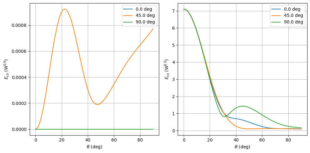
Data in nearfield grids
In the nearfield, generally there are three non-trivial field components. Recall the definition of the coordinates and according to Eq. 1 and Figure 1.
fig, ax = gridplot_magnitudes(da_grid_efield.sel(freq=da_grid_efield.freq.values[0]))
plt.tight_layout()
plt.show()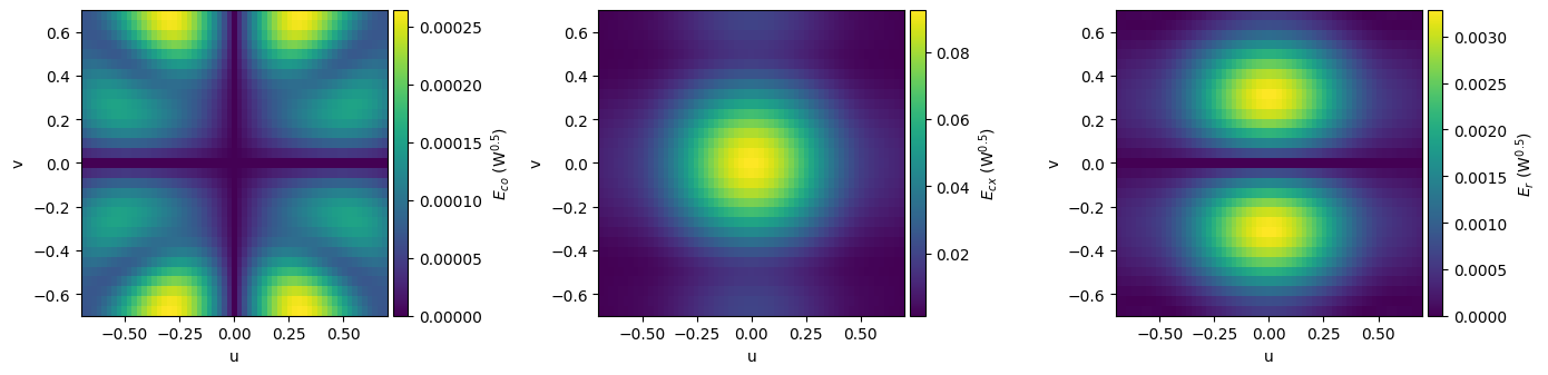
- Schmid, P. J., Sartori, M., Gabella, M., Renker, M., Wolfensberger, D., Kotiranta, M., & Murk, A. (2025). Scattering parameters of a wet radome. International Journal of Microwave and Wireless Technologies, 17(5), 862–873. 10.1017/S1759078725000546
- TICRA Tools User’s Manual (24.1). (2024). TICRA.